Urban footprinter: a repeatable convolution-based approach to extract urban extents from land use/land cover rasters

This post is a description of the urban-footprinter package, derived from its overview notebook, which can be executed interactively in your browser via myBinder by following this link.

Administrative boundaries are often defined manually case-by-case and based on subjective judgement. As a consequence, their widespread use in the context of urban and enviornmental studies can lead to misleading outcomes [1, 2].

The aim of the urban footprinter package is to provide a repeatable convolution-based method to extract the extent of the urban regions.

The study area for this example is a rasterized extract of the official cadastral survey of the Canton of Zurich, Switzerland.

import matplotlib.pyplot as plt
import numpy as np
import rasterio as rio
from matplotlib import cm, colors
from scipy import ndimage as ndi

import urban_footprinter as ufp


raster_filepath = 'data/zurich.tif'

with rio.open(raster_filepath) as src:
    lulc_arr = src.read(1)
    res = src.res[0]  # only square pixels are supported

    # custom colormap to plot the raster
    # https://matplotlib.org/3.1.1/tutorials/colors/colormap-manipulation.html
    num_classes = len(np.unique(lulc_arr))
    terrain_r_cmap = cm.get_cmap('terrain_r', num_classes)
    color_values = terrain_r_cmap(np.linspace(0, 1, num_classes))
    blue = np.array([0, .8, 1, 1])
    color_values[13, :] = blue  # water
    color_values[14, :] = blue  # water
    cmap = colors.ListedColormap(color_values)

    # np.where is used because nodata values of 255 would distort the colormap
    plt.imshow(np.where(lulc_arr != 255, lulc_arr, -1), cmap=cmap)
    plt.colorbar()

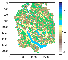
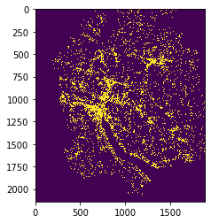
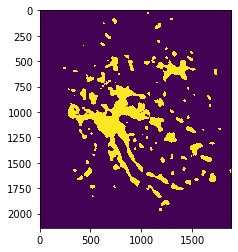
According to the land cover classification of the dataset, the codes 0 to 7 correspond to urban land cover classes. Therefore, the array of urban/non-urban pixels looks as follows:

urban_lulc_classes = range(8)
urban_lulc_arr = np.isin(lulc_arr, urban_lulc_classes).astype(np.uint32)

plt.imshow(urban_lulc_arr)

How the urban footprinter works

The approach of the urban footprinter library is built upon the methods used in the “Atlas of Urban Expansion” by Angel et al. [3]. The main idea is that a pixel is considered part of the urban extent depending on the proportion of built-up pixels that surround it. Accordingly, the extraction of the urban extent can be customized by means of the following three parameters:

• kernel_radius: radius (in meters) of the circular kernel used in the convolution
• urban_threshold: proportion of neighboring (within the kernel) urban pixels after which a given pixel is considered urban
• buffer_dist (optional): buffer distance (in meters) to add around the computed mask

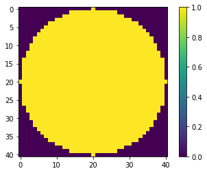
Convolution with a circular kernel

The main task consists in computing, for each pixel of the raster, the proportion of surrounding build-up pixels. This is done by means of a convolution with a circular kernel. In this example, the kernel_radius parameter will be set to 500 meters.

kernel_radius = 500

kernel_pixel_radius = int(kernel_radius // res)
kernel_pixel_len = 2 * kernel_pixel_radius + 1

y, x = np.ogrid[-kernel_pixel_radius:kernel_pixel_len -
                kernel_pixel_radius, -kernel_pixel_radius:
                kernel_pixel_len - kernel_pixel_radius]
mask = x * x + y * y <= kernel_pixel_radius * kernel_pixel_radius

kernel = np.zeros((kernel_pixel_len, kernel_pixel_len), dtype=np.uint32)
kernel[mask] = 1

The kernel will be an array of ones (the circle) and zeros which looks as follows:

plt.imshow(kernel)
plt.colorbar()

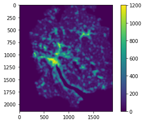
The convolution is computed by means of the convolve function of SciPy.

conv_result = ndi.convolve(urban_lulc_arr, kernel)

Since both urban_lulc_arr and kernel are arrays of ones and zeros, the result corresponds to the number of built-up pixels that lie within a 500m distance.

plt.imshow(conv_result)
plt.colorbar()

Filtering the convolution results

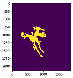
The result of the convolution is then used to classify pixels that are part of the urban extent. To this end, the urban_threshold parameter sets the proportion of surrounding built-up pixels after which a pixel is to be considered part of the urban extent. In this example, it will be set to 0.25 (i.e., 25%).

urban_threshold = 0.25

urban_mask = conv_result >= urban_threshold * np.sum(kernel)

The result looks as follows:

plt.imshow(urban_mask)

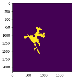
Optional: extract only the largest urban cluster

The fact that raster images are rectangular and real-world cities are not often entails that the raster includes more than just one urban settlement. In such case, the user might be interested in the extent that corresponds to the main urban settlement, namely, the largest urban patch of the raster. The largest urban cluster of the resulting urban_mask can be obtained by means of the label function of SciPy, which performs a connected-component labeling of the input array (i.e., urban_mask).

kernel_moore = ndi.generate_binary_structure(2, 2)
label_arr = ndi.label(urban_mask, kernel_moore)[0]
cluster_label = np.argmax(np.unique(label_arr, return_counts=True)[1][1:]) + 1
urban_mask = (label_arr == cluster_label).astype(np.uint8)

which produces the following output:

plt.imshow(urban_mask)

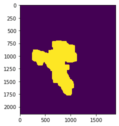
Optional: adding a buffer around the mask

In some contexts, e.g., the study of the urban-rural gradient in landscape ecology, it might be of interest to add a buffer around the urban extent. In this example, a buffer of 1000 meters will be added to the extracted urban extent. To this end, the binary_dilation function of Scipy can be used as follows:

buffer_dist = 1000

iterations = int(buffer_dist // res)
kernel_moore = ndi.generate_binary_structure(2, 2)
urban_mask = ndi.binary_dilation(
    urban_mask, kernel_moore, iterations=iterations)

which produces the following output:

plt.imshow(urban_mask)

The urban footprinter API

In the urban footprinter package, the procedure described above is encapsulated into a single function named urban_footprint_mask, which accepts the following arguments:

help(ufp.urban_footprint_mask)

Help on function urban_footprint_mask in module urban_footprinter:

urban_footprint_mask(raster, kernel_radius, urban_threshold, urban_classes=None, largest_patch_only=True, buffer_dist=None, res=None)
    Computes a boolean mask of the urban footprint of a given raster.

    Parameters
    ----------
    raster : ndarray or str, file object or pathlib.Path object
        Land use/land cover (LULC) raster. If passing a ndarray (instead of the
        path to a geotiff), the resolution (in meters) must be passed to the
        `res` keyword argument.
    kernel_radius : numeric
        The radius (in meters) of the circular kernel used in the convolution.
    urban_threshold : float from 0 to 1
        Proportion of neighboring (within the kernel) urban pixels after which
        a given pixel is considered urban.
    urban_classes : int or list-like, optional
        Code or codes of the LULC classes that must be considered urban. Not
        needed if `raster` is already a boolean array of urban/non-urban LULC
        classes.
    largest_patch_only : boolean, default True
        Whether the returned urban/non-urban mask should feature only the
        largest urban patch.
    buffer_dist : numeric, optional
        Distance to be buffered around the urban/non-urban mask. If no value is
        provided, no buffer is applied.
    res : numeric, optional
        Resolution of the `raster` (assumes square pixels). Ignored if `raster`
        is a path to a geotiff.

    Returns
    -------
    urban_mask : ndarray

kernel_radius = 500
urban_threshold = 0.25
urban_classes = list(range(8))

Therefore, the urban extent extracted above can be obtained as in:

urban_mask = ufp.urban_footprint_mask(raster_filepath,
                                      kernel_radius,
                                      urban_threshold,
                                      urban_classes=urban_classes)

plt.imshow(urban_mask)

Alternatively, the urban extent can also be obtained as a vector geometry (instead of a raster array) by means of the urban_footprint_mask_shp function:

urban_mask = ufp.urban_footprint_mask_shp(raster_filepath,
                                          kernel_radius,
                                          urban_threshold,
                                          urban_classes=urban_classes)

urban_mask

References

1. Oliveira, E. A., Andrade Jr, J. S., & Makse, H. A. (2014). Large cities are less green. Scientific reports, 4, 4235.
2. Rozenfeld, H. D., Rybski, D., Andrade, J. S., Batty, M., Stanley, H. E., & Makse, H. A. (2008). Laws of population growth. Proceedings of the National Academy of Sciences, 105(48), 18702-18707.
3. Angel, S., Blei, A. M., Civco, D. L., & Parent, J. (2016). Atlas of urban expansion - The 2016 edition, Volume 1: Areas and Densities. New York: New York University, Nairobi: UN-Habitat, and Cambridge, MA: Lincoln Institute of Land Policy.

Martí Bosch

Urban sprawl, Python, and a bit of landscape ecology and complexity

Tweet Share