On spatial joins between networks and polygon geometries in Python
- 21 minsA Jupyter notebook with the whole code materials used is available at martibosch.github.io/blob/master/assets/notebooks/network_spatial_joins.ipynb
The research of my colleague Armel Kemajou focuses on how informal transportation is shaping suburbanization in Sub-Saharan Africa. To that end, he performed a field survey to collect a GPS traces of a sample of mototaxi drivers in the cities Yaoundé, Cameroon and Lomé, Togo (some results in Yaoundé have already been published as a journal article). In order to address to what extent such emerging means of transportations pave the way for urban sprawl, it is crucial to explore the characteristics of the origin and destination locations of each trip. Among other questions, we were therefore interested in the evaluating how developed is the street network around the destination locations.
After some preprocessing of the GPS traces in Yaoundé, we have a CSV file with the locations and times of the origins and destinations of 23712 trips during three weeks. For the sake of simplicity, let us consider only the 8943 trips whose destination falls within the longitudes of 3.8° and 3.85° and the latitudes of 11.4° and 11.5°. We then have a geo-data frame of the following form:
trip_gdf.head()
| origin_dt | dest_dt | neighborhood | origin | dest | |
|---|---|---|---|---|---|
| 415 | 2018-02-07 09:01:12 | 2018-02-07 09:45:09 | Nkozoa | POINT (11.540371 3.965306) | POINT (11.47033 3.83131) |
| 416 | 2018-02-07 12:06:37 | 2018-02-07 12:13:16 | Nkozoa | POINT (11.471801 3.834358) | POINT (11.48885 3.83186) |
| 422 | 2018-02-07 13:52:37 | 2018-02-07 14:15:07 | Nkozoa | POINT (11.504751 3.867998) | POINT (11.47140 3.82584) |
| 423 | 2018-02-07 14:17:26 | 2018-02-07 14:22:03 | Nkozoa | POINT (11.471725 3.824733) | POINT (11.45961 3.80135) |
| 424 | 2018-02-07 15:08:45 | 2018-02-07 15:22:56 | Nkozoa | POINT (11.459691 3.80134) | POINT (11.48888 3.83142) |
Let us then use OSMnx to get the street network ot the area:
# get convex hull in lat/long to query OSM
convex_hull = trip_gdf['dest'].unary_union.convex_hull
# get the street network and project it
G = ox.graph_from_polygon(convex_hull, network_type='drive')
# the undirected graph will do for our purposes
G = ox.project_graph(G.to_undirected(reciprocal=False))
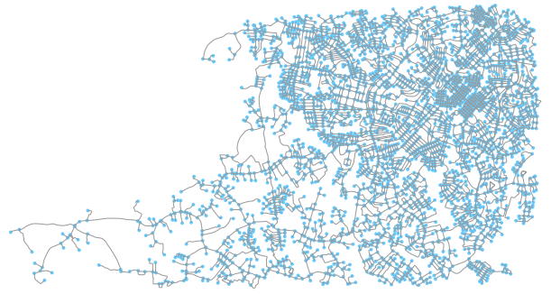
We obtain a network of 4032 nodes and 5344 edges which looks as follows:
fig, ax = ox.plot_graph(G)
Using the trips geo-data frame and the street network shown above, we want to compute, for each of the trip destinations, the total street length that falls within a 100 m radius of the destination location. Let us use the code snippet below to illustrate the situation:
# let us first reproject `trip_gdf` to the network's CRS
dest_gdf = gpd.GeoDataFrame(geometry=trip_gdf['dest'])
dest_gdf.crs = 'epsg:4326'
trip_gdf['dest'] = ox.project_gdf(loc_gdf)

# select the destination point of the first trip
point = trip_gdf.iloc[0]['dest']
point_buffer = point.buffer(buffer_dist)

fig, ax = ox.plot_graph(G, show=False, close=False)
ax.plot(point.x, point.y, 'x', color='r')
ax.plot(*point_buffer.exterior.xy, color='g')
plt.show()
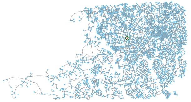
Therefore, for each trip, we need to truncate the street network to the extent of the 100 m buffer around its destination location. To that end, we might use the truncate_graph_polygon funcion of OSMnx as in the code snippet below:
def get_buffer_street_length(point, buffer_dist, G):
    geom = point.buffer(buffer_dist)
    try:
        buffer_G = ox.truncate_graph_polygon(
            G, geom, truncate_by_edge=True, retain_all=True)
        return sum([d['length'] for u, v, d in buffer_G.edges(data=True)])
    except:
        return 0
which we can then call by providing the point variable defined above, i.e., the location of the destination of the first trip, a buffer distance of 100 m, and the projected street network G as in:
street_length = get_buffer_street_length(point, 100, G)
Nevertheless, the such call takes 19.4 s in my Lenovo X1C6 laptop, which is clearly too slow considering that we need to perform such computation for each of the 8943 trips.
First step: spatial join
There are two main issues that we need to address regarding the performance of our code.
- Asymptotic complexity: for each of our K trips, we need to test which of the N nodes fall within the 100 m radius of the destination location. A brute force algorithm would require $\mathcal{O}(K \cdot N)$. In order to improve that, we can use a tree-based spatial indexing such as an R-tree. This post by Geoff Boeing uses Python and GeoPandas to provide a nice overview of its advantages. Making use of such techniques can improve the asymptotic complexity to $\mathcal{O}((K + N) \cdot log(K) + f)$, where f is the number of interesections between minimum bounding rectangles found1. Long story short, such gain becomes key when we deal with large datasets.
- Dynamic typing and interpreted execution in Python: Python is an interpreted language which is prone to significant execution overheads because of its dynamic type-checking. In short, this means that you should avoid iterating over large arrays and instead operate with NumPy typed arrays with ufuncs, aggregates (e.g.,
np.mean,np.max, …), slicing, masking and the like.
In Python, both issues can be addressed by making use of the spatial join operation of GeoPandas2. To that end, we need to prepare two geo-data frames, i.e., a first one where the destination points of each trip are transformed into polygon geometries representing the circular buffers with a 100 m radius, and a second one with the point geometries of each node of the street network:
# left geo-data frame
# add a buffer around the point geometries
buffer_gdf = gpd.GeoDataFrame(
    geometry=trip_gdf['dest'].apply(lambda p: p.buffer(buffer_dist)),
    index=trip_gdf.index)
buffer_gdf.crs = G.graph['crs']

# right geo-data frame
# get list of nodes from the projected graph
node_geom = [
    geometry.Point(data['x'], data['y']) for _, data in G.nodes(data=True)
]
# create a GeoDataFrame with the node ids and their point geometries
node_gdf = gpd.GeoDataFrame(
    {
        'node': pd.Series(G.nodes()),
        'geometry': node_geom
    }, crs=G.graph['crs'])
Then we can perform the spatial join as in:
sjoin_gdf = gpd.sjoin(buffer_gdf, node_gdf, op='contains')
which will test, whether each buffer geometry of buffer_gdf contains the nodes of the street network represented in node_gdf. Since the resulting sjoin_gdf will have the same index as its first argument (i.e., the id of each buffer geometry, thus the id of each trip), we can use a group-by operation as in:
for trip_index, group_gdf in sjoin_gdf.groupby(sjoin_gdf.index):
    break  # here we just want to see the first group
which will, for each buffer geometry, yield a geo-data frame of the form:
group_gdf
| geometry | index_right | node | |
|---|---|---|---|
| 415 | POLYGON ((774460.018 423876.374, 774459.536 42... | 619 | 5795317038 |
| 415 | POLYGON ((774460.018 423876.374, 774459.536 42... | 2962 | 2322601884 |
| 415 | POLYGON ((774460.018 423876.374, 774459.536 42... | 2970 | 2322601912 |
| 415 | POLYGON ((774460.018 423876.374, 774459.536 42... | 2974 | 2322601917 |
Note that the index and geometry column are the same since they correspond to the same buffer geometry (i.e., and in turn to the same trip), and therefore the node column shows us which nodes of node_gdf are inside such buffer geometry.
Compute the street length with group by and apply
Given the result of the spatial join, we can use the G.subgraph method of NetworkX to get the subgraph that corresponds to the set of nodes each group_gdf, i.e.:
G.subgraph(group_gdf['node'])
In our case, in order to compute the street length of each buffer, we first need to define a function that will be called for each group data frame (such as the one shown above) of the group-by operation. Consider the following snippet:
# get street length
# first define function to compute street length given a list of nodes
# from G that fall within the buffer extent
def get_street_length(nodes, G):
    buffer_G = G.subgraph(nodes)
    return sum([
        d['length'] for u, v, d in buffer_G.edges(data=True)
    ])
Then we can compute the street length of each trip (remember that the elements of sjoin_gdf are indexed by the trip ids) as in:
trip_gdf['street_length'] = sjoin_gdf['node'].groupby(
    sjoin_gdf.index).apply(get_street_length, G)
There might be trips where their respective buffer geometry does not contain any graph node, which will be represented by a nan value (after the column assignment of the code snippet above). Since this means that no nodes of the street networks are found around the trip destination, we can fill such rows of trip_gdf with a 0.
trip_gdf['street_length'] = trip_gdf['street_length'].fillna(0)
For the 8943 trips, the combination of (i) the spatial join, (ii) group-by computation of the street length and (iii) filling nan values takes a total of 2.66 s in my laptop.
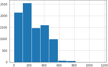
We can now plot our distribution of street lengths as in:
_ = trips_df['street_length'].hist()
Going one step further: including incomplete street segments
Although the computational workflow described above has provided us with a distribution of street lenghts in satisfactory time, it has a key conceptual shortcoming. Let us illustrate it by plotting the subgraph that correspond group_gdf used above:
fig, ax = ox.plot_graph(G.subgraph(group_gdf['node']),
                        margin=2,
                        show=False,
                        close=False)
ax.plot(point.x, point.y, 'x', color='r')
ax.plot(*point_buffer.exterior.xy, color='g')
plt.show()
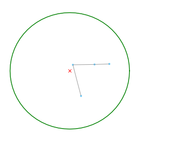
As we can observe, the subgraph method returns a graph with only those nodes that are inside the buffer geometry and the edges between them. This might make sense for networks whose edges represent ethereal connections (e.g., social networks), but in networks whose edges represent physical connections (e.g., streets), we might be interested in retaining the edge segments that fall within the buffer geometry. To make such a point more clear, compare the subgraph plot above with the one below:
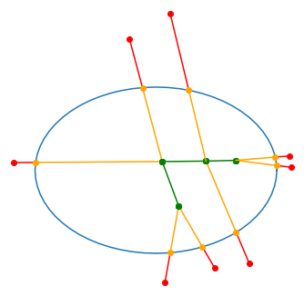
The edges are colored in green when they link the green nodes, i.e., those that are inside the buffer geometry, like the graph returned by the subgraph method. The red nodes are nodes from the street network that are outside the buffer geometry but link to a node inside it (i.e., the red edges). The orange nodes, which are not originally in the street network, represent the intersection between the red edges and the boundaries of the buffer geometry. Finally, the orange edges (which overlay part of the red edges) represent the street segments that lie inside the buffer zones but lead to a node that is outside of it.
It seems clear that such orange segments must be considered in order to obtain a fair impression of the characteristics of the street network inside each buffer zone. It seems rather hasty to assume beforehand that ommiting them has no significant effect over the resulting distribution of street lenghts or that such residuals will be normally distributed.
To obtain the orange segments, we can use the G.edges method, which takes as argument a list of nodes in G, and returns those edges that involve at least one of such nodes. We will then distinguish between two main cases: (a) edges such that both nodes are inside the buffer geometry (i.e., the green edges above) and (b) edges a node inside the buffer geometry and the other outisde it (i.e., the red edges above). In the latter case, we will use Shapely to get the interception between such edges and the boundaries of the buffer geometry (i.e., the orange nodes), and then add a synthetic edge between the inner node and the interception (i.e., the orange edges). Let us wrap the foregoing concepts into a function that can be called at each iteration of a group by loop as in:
def get_graph_in_geom(geom, nodes, G):
    # prepare the new graph
    # the `MultiGraph` type and the 'crs' and 'name' attributes are needed
    # to plot with osmnx
    G_in_geom = nx.MultiGraph()
    for attr_key in ['crs', 'name']:
        G_in_geom.graph[attr_key] = G.graph[attr_key]
    G_in_geom.add_nodes_from(G.subgraph(nodes).nodes(data=True))

    # iterate over all the edges that involve at least one node of `nodes`
    for u, v, d in G.edges(nodes, data=True):
        node_u = G.nodes[u]
        node_v = G.nodes[v]
        p_u = geometry.Point(node_u['x'], node_u['y'])
        p_v = geometry.Point(node_v['x'], node_v['y'])
        if p_u.within(geom):
            if p_v.within(geom):
                # both nodes are inside `geom`
                G_in_geom.add_edge(u, v, length=d['length'])
                continue
            else:
                # `u` is inside `geom` but `v` is outside
                node_in_id, node_out_id = node_u['osmid'], node_v['osmid']
                p_in, p_out = p_u, p_v
        else:
            # since the argument `nodes` (that we pass to `subgraph`
            # above) comes from the spatial join we know that at least one
            # node is inside `geom`
            # `v` is inside `geom` but `u` is outside
            node_in_id, node_out_id = node_v['osmid'], node_u['osmid']
            p_in, p_out = p_v, p_u

        # if we get here, it is because we have `p_in` inside `geom` and
        # `p_out` outside, otherwise (i.e., both nodes inside `geom`) the
        # `continue` statement would have brought us directly to the next
        # iteration
        intercept = geom.boundary.intersection(
            geometry.LineString([p_in, p_out]))

        # compute the distance between the node inside `geom` and the
        # interception between the edge and `geom`
        dist = p_in.distance(intercept)
        # add the node for the interception with the same id as the node
        # that is outside of `geom`
        G_in_geom.add_node(node_out_id, x=intercept.x, y=intercept.y)
        # add an edge from the node inside `geom` to the interception
        G_in_geom.add_edge(node_in_id, node_out_id, length=dist)

    return G_in_geom
Then we can finish our spatial join as in (note that using tqdm to display a progress bar is optional):
G_list = []
for trip_index, group_gdf in notebook.tqdm(
        sjoin_gdf.groupby(sjoin_gdf.index)):
    buffer_geom = group_gdf.iloc[0]['geometry']
    nodes = group_gdf['node']

    G_in_geom = get_graph_in_geom(buffer_geom, nodes, G)
    G_list.append(G_in_geom)
which will return a list of the graphs G_list where each position matches the index of trip_gdf features a NetworkX graph instance representing the street network inside the 100 m buffer around the destination of each trip. The execution of the above snippet takes 26.2 s in my laptop.
We can now compute the street length of each graph very easily with a function such as:
def compute_street_length(G):
    return sum([d['length'] for u, v, d in G.edges(data=True)])
which can be used in a loop as in:
street_lengths = []
for G_in_geom in notebook.tqdm(G_list):
    street_lengths.append(compute_street_length(G_in_geom))
and takes 395 ms in my laptop. We can now plot the difference between the two approaches:
figwidth, figheight = plt.rcParams['figure.figsize']
fig, (ax_l, ax_r) = plt.subplots(1, 2, figsize=(2 * figwidth, figheight))

# left plot
alpha = 0.7  # to overlay histograms
trip_gdf['street_length'].hist(alpha=alpha, label='inner only', ax=ax_l)
street_length_ser.hist(alpha=alpha, label='intercept', ax=ax_l)
ax_l.legend()
ax_l.set_title('Street lengths')

# right plot
(trip_gdf['street_length'] - street_length_ser).hist(ax=ax_r)
ax_r.set_title('Differences')
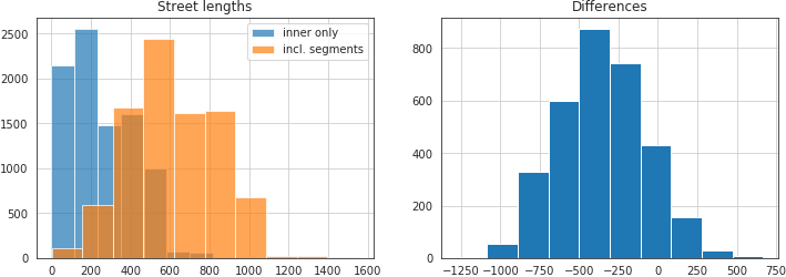
As noted in the left plot, the distribution of street lengths when considering the inner edges only and when including the street segments are quite different. From the plot in the right, we can see that such differences follow a normal distribution centered at -355.92 m.
On further performance improvements
The 26 s required to include the incomplete street segments in our spatial join is significantly slower than the 2.66 seconds required when ommiting them. Nonetheless, there is still room for many performance improvements. Firstly, the group by for loop where we call get_graph_in_geom is embarrassingly parallel, and therefore can easily be performed at scale with Dask. Secondly, NetworkX is a rather slow library to model networks when compared to other Python alternatives such as graph-tool or igraph. Thirdly, the geometric operations that we perform with shapely (i.e., interception of the red edges and the boundaries of the buffer geometries) are relatively simple and could be implemented with NumPy to avoid overheads. Finally, there exists a set of libraries that allow us to compile our Python code into faster machine languages and significantly improve the execution speeds e.g., Cython, Numba, Pythran…
I might at some point amend this blog post with the implementation of some of the ideas listed above. In the meantime, the proposed approach allows us to comfortably operate on networks of some thousand nodes in a laptop.
Notes
-
See Jacox, E. H., & Samet, H. (2007). Spatial join techniques. ACM Transactions on Database Systems (TODS), 32(1), 7-es. ↩
-
Actually, some geometry operations in GeoPandas used to be slow because the geometry elements were stored as a generic
object-dtype column with Shapely objects. To improve that, an initial idea by Joris Van den Bossche consisted in changing theobject-dtype gometry column for a NumPy array of pointers to GEOS objects. It seems that such an approach has been put aside and the GeoPandas developers in favor of making use of the spatial operations from the PyGEOS package, although the latter is still experimental. In any case, the spatial join of GeoPandas employed in this article was already Cythonized by Matthew Rocklin in August 2017, so I do not know whether preformance improvements are to be expected in such operation. ↩
